Convolutional Neural Networks, Section 2
Convolutional Layer
The Conv layer is the core building block of a Convolutional Network that does most of the computational heavy lifting.
Overview and intuition without brain stuff. Lets first discuss what the CONV layer computes without brain/neuron analogies. The CONV layer’s parameters consist of a set of learnable filters. Every filter is small spatially (along width and height), but extends through the full depth of the input volume. For example, a typical filter on a first layer of a ConvNet might have size 5x5x3 (i.e., 5 pixels width and height, and 3 because images have depth 3, the color channels).
During the forward pass, we slide (more precisely, convolve) each filter across the width and height of the input volume and compute dot products between the entries of the filter and the input at any position. As we slide the filter over the width and height of the input volume we will produce a two-dimensional activation map that gives the responses of that filter at every spatial position. Intuitively, the network will learn filters that activate when they see some type of visual feature such as an edge of some orientation or a blotch of some color on the first layer, or eventually entire honeycomb or wheel-like patterns on higher layers of the network. Now, we will have an entire set of filters in each CONV layer (e.g., 12 filters), and each of them will produce a separate two-dimensional activation map. We will stack these activation maps along the depth dimension and produce the output volume.
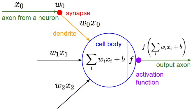
The brain view. If you’re a fan of the brain/neuron analogies, every entry in the 3D output volume can also be interpreted as an output of a neuron that looks at only a small region in the input and shares parameters with all neurons to the left and right spatially (since these numbers all result from applying the same filter). We now discuss the details of the neuron connectivities, their arrangement in space, and their parameter sharing scheme.
Local Connectivity. When dealing with high-dimensional inputs such as images, as we saw above it is impractical to connect neurons to all neurons in the previous volume. Instead, we will connect each neuron to only a local region of the input volume. The spatial extent of this connectivity is a hyperparameter called the receptive field of the neuron (equivalently this is the filter size). The extent of the connectivity along the depth axis is always equal to the depth of the input volume. It is important to emphasize again this asymmetry in how we treat the spatial dimensions (width and height) and the depth dimension: The connections are local in space (along width and height), but always full along the entire depth of the input volume.
Example 1. For example, suppose that the input volume has size [32x32x3], (e.g., an RGB CIFAR-10 image). If the receptive field (or the filter size) is 5×5, then each neuron in the Conv Layer will have weights to a [5x5x3] region in the input volume, for a total of 5*5*3 = 75 weights (and +1 bias parameter). Notice that the extent of the connectivity along the depth axis must be 3, since this is the depth of the input volume.
Example 2. Suppose an input volume had size [16x16x20]. Then using an example receptive field size of 3×3, every neuron in the Conv Layer would now have a total of 3*3*20 = 180 connections to the input volume. Notice that, again, the connectivity is local in space (e.g., 3×3), but full along the input depth (20).
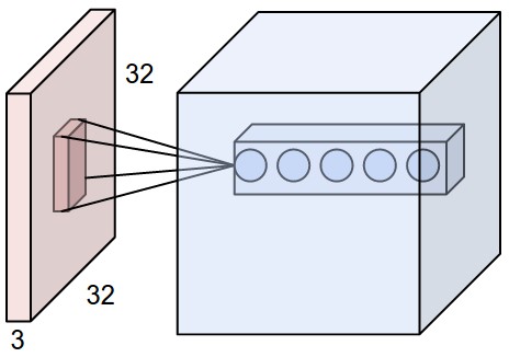
Left: An example input volume in red (e.g. a 32x32x3 CIFAR-10 image), and an example volume of neurons in the first convolutional layer. Each neuron in the convolutional layer is connected only to a local region in the input volume spatially, but to the full depth (i.e., all color channels). Note, there are multiple neurons (5 in this example) along the depth, all looking at the same region in the input – see discussion of depth columns in text below. Right: The neurons from the Neural Network chapter remain unchanged: They still compute a dot product of their weights with the input followed by a non-linearity, but their connectivity is now restricted to be local spatially.
Spatial arrangement. We have explained the connectivity of each neuron in the Conv Layer to the input volume, but we haven’t yet discussed how many neurons there are in the output volume or how they are arranged. Three hyperparameters control the size of the output volume: the depth, stride and zero-padding. We discuss these next:
- First, the depth of the output volume is a hyperparameter: it corresponds to the number of filters we would like to use, each learning to look for something different in the input. For example, if the first convolutional layer takes as input the raw image, then different neurons along the depth dimension may activate in presence of various oriented edges, or blobs of color. We will refer to a set of neurons that are all looking at the same region of the input as a depth column (some people also prefer the term fibre).
- Second, we must specify the stride with which we slide the filter. When the stride is 1 then we move the filters one pixel at a time. When the stride is 2 (or uncommonly 3 or more, though this is rare in practice) then the filters jump 2 pixels at a time as we slide them around. This will produce smaller output volumes spatially.
- As we will soon see, sometimes it will be convenient to pad the input volume with zeros around the border. The size of this zero-padding is a hyperparameter. The nice feature of zero padding is that it will allow us to control the spatial size of the output volumes (most commonly as we’ll see soon we will use it to exactly preserve the spatial size of the input volume so the input and output width and height are the same).
We can compute the spatial size of the output volume as a function of the input volume size (W), the receptive field size of the Conv Layer neurons (F), the stride with which they are applied (S), and the amount of zero padding used (P) on the border. You can convince yourself that the correct formula for calculating how many neurons “fit” is given by (W−F+2P)/S+1. For example for a 7×7 input and a 3×3 filter with stride 1 and pad 0 we would get a 5×5 output. With stride 2 we would get a 3×3 output. Let’s also see one more graphical example:

Illustration of spatial arrangement. In this example there is only one spatial dimension (x-axis), one neuron with a receptive field size of F = 3, the input size is W = 5, and there is zero padding of P = 1. Left: The neuron strided across the input in stride of S = 1, giving output of size (5 – 3 + 2)/1+1 = 5. Right: The neuron uses stride of S = 2, giving output of size (5 – 3 + 2)/2+1 = 3. Notice that stride S = 3 could not be used since it wouldn’t fit neatly across the volume. In terms of the equation, this can be determined since (5 – 3 + 2) = 4 is not divisible by 3. The neuron weights are in this example [1,0,-1] (shown on very right), and its bias is zero. These weights are shared across all yellow neurons (see parameter sharing below).
Use of zero-padding. In the example above on left, note that the input dimension was 5 and the output dimension was equal: also 5. This worked out so because our receptive fields were 3 and we used zero padding of 1. If there was no zero-padding used, then the output volume would have had spatial dimension of only 3, because that it is how many neurons would have “fit” across the original input. In general, setting zero padding to be P=(F−1)/2 when the stride is S=1 ensures that the input volume and output volume will have the same size spatially. It is very common to use zero-padding in this way and we will discuss the full reasons when we talk more about ConvNet architectures.
Constraints on strides. Note again that the spatial arrangement hyperparameters have mutual constraints. For example, when the input has size W=10, no zero-padding is used P=0, and the filter size is F=3, then it would be impossible to use stride S=2, since (W−F+2P)/S+1=(10−3+0)/2+1=4.5, i.e., not an integer, indicating that the neurons don’t “fit” neatly and symmetrically across the input. Therefore, this setting of the hyperparameters is considered to be invalid, and a ConvNet library could throw an exception or zero pad the rest to make it fit, or crop the input to make it fit, or something. As we will see in the ConvNet architectures section, sizing the ConvNets appropriately so that all the dimensions “work out” can be a real headache, which the use of zero-padding and some design guidelines will significantly alleviate.
Real-world example. The Krizhevsky et al. architecture that won the ImageNet challenge in 2012 accepted images of size [227x227x3]. On the first Convolutional Layer, it used neurons with receptive field size F=11, stride S=4 and no zero padding P=0. Since (227 – 11)/4 + 1 = 55, and since the Conv layer had a depth of K=96, the Conv layer output volume had size [55x55x96]. Each of the 55*55*96 neurons in this volume was connected to a region of size [11x11x3] in the input volume. Moreover, all 96 neurons in each depth column are connected to the same [11x11x3] region of the input, but of course with different weights. As a fun aside, if you read the actual paper it claims that the input images were 224×224, which is surely incorrect because (224 – 11)/4 + 1 is quite clearly not an integer. This has confused many people in the history of ConvNets and little is known about what happened. My own best guess is that Alex used zero-padding of three extra pixels that he does not mention in the paper.
Parameter Sharing. Parameter sharing scheme is used in Convolutional Layers to control the number of parameters. Using the real-world example above, we see that there are 55*55*96 = 290,400 neurons in the first Conv Layer, and each has 11*11*3 = 363 weights and 1 bias. Together, this adds up to 290400 * 364 = 105,705,600 parameters on the first layer of the ConvNet alone. Clearly, this number is very high.
It turns out that we can dramatically reduce the number of parameters by making one reasonable assumption: That if one feature is useful to compute at some spatial position (x,y), then it should also be useful to compute at a different position (x2,y2). In other words, denoting a single 2-dimensional slice of depth as a depth slice (e.g., a volume of size [55x55x96] has 96 depth slices, each of size [55×55]), we are going to constrain the neurons in each depth slice to use the same weights and bias. With this parameter sharing scheme, the first Conv Layer in our example would now have only 96 unique set of weights (one for each depth slice), for a total of 96*11*11*3 = 34,848 unique weights, or 34,944 parameters (+96 biases). Alternatively, all 55*55 neurons in each depth slice will now be using the same parameters. In practice during backpropagation, every neuron in the volume will compute the gradient for its weights, but these gradients will be added up across each depth slice and only update a single set of weights per slice.
Notice that if all neurons in a single depth slice are using the same weight vector, then the forward pass of the CONV layer can in each depth slice be computed as a convolution of the neuron’s weights with the input volume (Hence the name: Convolutional Layer). This is why it is common to refer to the sets of weights as a filter (or a kernel), that is convolved with the input.
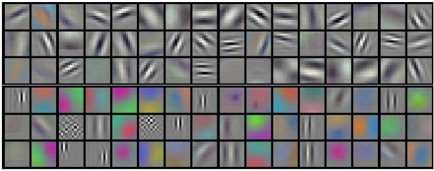
Example filters learned by Krizhevsky et al. Each of the 96 filters shown here is of size [11x11x3], and each one is shared by the 55*55 neurons in one depth slice. Notice that the parameter sharing assumption is relatively reasonable: If detecting a horizontal edge is important at some location in the image, it should intuitively be useful at some other location as well due to the translationally-invariant structure of images. There is therefore no need to relearn to detect a horizontal edge at every one of the 55*55 distinct locations in the Conv layer output volume.
Note that sometimes the parameter sharing assumption may not make sense. This is especially the case when the input images to a ConvNet have some specific centered structure, where we should expect, for example, that completely different features should be learned on one side of the image than another. One practical example is when the input are faces that have been centered in the image. You might expect that different eye-specific or hair-specific features could (and should) be learned in different spatial locations. In that case it is common to relax the parameter sharing scheme, and instead simply call the layer a Locally-Connected Layer.
Numpy examples. To make the discussion above more concrete, lets express the same ideas but in code and with a specific example. Suppose that the input volume is a numpy array X. Then:
- A depth column (or a fibre) at position
(x,y)would be the activationsX[x,y,:]. - A depth slice, or equivalently an activation map at depth
dwould be the activationsX[:,:,d].
Conv Layer Example. Suppose that the input volume X has shape X.shape: (11,11,4). Suppose further that we use no zero padding (P=0), that the filter size is F=5, and that the stride is S=2. The output volume would therefore have spatial size (11-5)/2+1 = 4, giving a volume with width and height of 4. The activation map in the output volume (call it V), would then look as follows (only some of the elements are computed in this example):
V[0,0,0] = np.sum(X[:5,:5,:] * W0) + b0V[1,0,0] = np.sum(X[2:7,:5,:] * W0) + b0V[2,0,0] = np.sum(X[4:9,:5,:] * W0) + b0V[3,0,0] = np.sum(X[6:11,:5,:] * W0) + b0
Remember that in numpy, the operation * above denotes elementwise multiplication between the arrays. Notice also that the weight vector W0 is the weight vector of that neuron and b0 is the bias. Here, W0 is assumed to be of shape W0.shape: (5,5,4), since the filter size is 5 and the depth of the input volume is 4. Notice that at each point, we are computing the dot product as seen before in ordinary neural networks. Also, we see that we are using the same weight and bias (due to parameter sharing), and where the dimensions along the width are increasing in steps of 2 (i.e. the stride). To construct a second activation map in the output volume, we would have:
V[0,0,1] = np.sum(X[:5,:5,:] * W1) + b1V[1,0,1] = np.sum(X[2:7,:5,:] * W1) + b1V[2,0,1] = np.sum(X[4:9,:5,:] * W1) + b1V[3,0,1] = np.sum(X[6:11,:5,:] * W1) + b1V[0,1,1] = np.sum(X[:5,2:7,:] * W1) + b1(example of going along y)V[2,3,1] = np.sum(X[4:9,6:11,:] * W1) + b1(or along both)
where we see that we are indexing into the second depth dimension in V (at index 1) because we are computing the second activation map, and that a different set of parameters (W1) is now used. In the example above, we are for brevity leaving out some of the other operations the Conv Layer would perform to fill the other parts of the output array V. Additionally, recall that these activation maps are often followed elementwise through an activation function such as ReLU, but this is not shown here.
Summary
To summarize, the Conv Layer:
- Accepts a volume of size W1×H1×D1
- Requires four hyperparameters:
- Number of filters K,
- their spatial extent F,
- the stride S,
- the amount of zero padding P.
- Produces a volume of size W2×H2×D2 where:
- W2=(W1−F+2P)/S+1
- H2=(H1−F+2P)/S+1 (i.e., width and height are computed equally by symmetry)
- D2=K
- With parameter sharing, it introduces F⋅F⋅D1 weights per filter, for a total of (F⋅F⋅D1)⋅K weights and K biases.
- In the output volume, the d-th depth slice (of size W2×H2) is the result of performing a valid convolution of the d-th filter over the input volume with a stride of S, and then offset by d-th bias.
A common setting of the hyperparameters is F=3,S=1,P=1. However, there are common conventions and rules of thumb that motivate these hyperparameters. We’ll cover these in the ConvNet architectures section in the next and final part of this series.
