

Machine learning is one of the most talked about fields in seemingly every industry spanning autonomous vehicles to health monitoring, financial management to education, robotics to biometrics, surveillance to home automation. Indeed, no industry will go untouched by the many machine learning technologies. The reasons for this boom are threefold: the maturation of the algorithms, the availability of inexpensive parallel processing power, and a massive amount of data—all conspiring to yield a big bang of development, and a perfect storm for the transformation of every imaginable application.
The series of articles in this special focus will not only provide a roadmap for learning the basic principles, but also provide the larger context of applications and impact that this bourgeoning technology is bringing to our world.
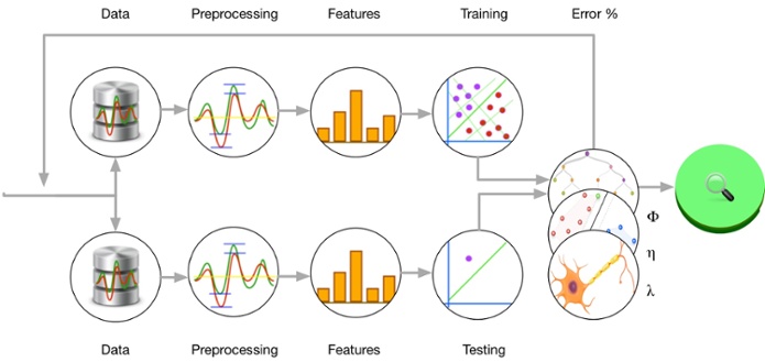
Thinking in Steps
Every machine learning problem tends to have its own particularities. Nevertheless, as the discipline advances, there are emerging patterns that suggest an ordered process to solving those problems. In this article, we’ll detail the main stages of this process, beginning with the conceptual understanding and culminating in a real world model evaluation.
Understanding the Problem
When solving machine learning problems, it’s important to take the time to analyze both the data and work ramifications beforehand. This preliminary step is flexible and less formal than all the subsequent steps we’ll cover.
From the definition of machine learning, we know that the final goal of our job is to make the computer learn, or generalize a determined behavior or model from a set of previously given data. So the first thing we should do is understand the new capabilities we want the model to learn.
The key questions we could ask ourselves during this phase might include:
- What is the real problem we are trying to solve?
- How is the current information pipeline configured?
- How can I streamline the data acquisition?
- Is the incoming data complete, or does it have “voids?”
- What additional data sources we could merge to generate more variables?
- Is the data periodical, or can it be acquired in real time?
- What is the minimal representative unit of time for this particular problem?
Understanding the problem often involves getting into the business intelligence side of the equation, and looking at all the valuable sources of information which could influence the model. Once identified, the next task is to generate an organized and structured set of values, which will be the input to our model. We call that group of data the dataset.
Dataset Definition and Retrieving
Once we have identified the data sources, the next task is to gather all the tuples or records as a homogeneous set. The format can be a tabular arrangement, a series of real values (audio, weather, or other variables of interest), N-Dimensional matrices (a set of images or cloud points), among other types. After this raw information is gathered, an enrichment stage follows, defined in a step called feature engineering.
Enriching and Pruning the Data
Feature engineering is in some ways one of the most underrated aspects of the machine learning process, even though it is considered the cornerstone of the learning process by many prominent figures in the AI community.
Simply stated, in this phase we take the raw data coming from databases, sensors, cameras, and other sources, and transform it in a way that makes easy for the model to generalize. This discipline takes criteria from many sources—including common sense. It is indeed more an art than a rigid science. It’s also a manual process, even when some parts of it can be automatized via techniques grouped in the feature extraction field.
Included in this process are many powerful mathematical tools, like the various dimensionality reductions techniques including PCA (Principal Component Analysis), Autoencoders, and others, which allow the data scientist to skip features that don’t enrich the representation of the data in useful ways.
Making Data Tractable: Dataset Preprocessing
When we first dive into data science, a common mistake is expecting all the data to be very polished and with nice characteristics from the very beginning. Alas, this is not the case for a very considerable percentage of situations for many reasons: the presence of null data, sensor errors that cause outliers and NAN, faulty registers, instrument-induced bias, and all kinds of other defects that lead to poor model fitting and must therefore be eradicated.
The two key processes in this stage are data normalization and feature scaling. These processes consist of applying simple transformations, called affine, which map the current unbalanced data into more manageable shape, maintaining its integrity while yielding better stochastic properties and improving the future applied model. The common goal of the standardization techniques is to bring the data distribution closer to a normal distribution of mean 0 and standard deviation of 1.
Model Definition
If we could summarize the machine learning process in just one word, it would certainly be models. This is because what we build with machine learning are abstractions or models representing and simplifying the reality, allowing us to solve real world problems, based on a model, which we trained accordingly.
The task of choosing which model to use is becoming increasingly difficult, given the increasing number of them appearing almost daily, but one can do general approximations, grouping methods by the type of tasks we want to do, and also the type of input data, so that the problem can simplified to a smaller set of options.
Asking the Right Questions
At risk of generalizing too much, let’s try to summarize a sample decision problem for a model:
- Are we trying to characterize data by simply grouping information based on its characteristics, without any or a few previous hints? This is the domain of clustering techniques.
- The first and most basic question: are we trying to predict the instant outcome of a variable, or we simply tagging or classifying data into groups? If the former, we are tackling a regression problem; if the latter, this is the realm of classification problems.
- Having resolved these questions, we ask, is the data sequential, or better, should we take the sequence into account? If so, then Recurrent Neural Networks should be one of our first options.
- Continuing with non-clustering techniques, is the data or patterns to discover spatially located? If so, then Convolutional Neural Networks are a common starting point.
- In the most common cases (data without a particular arrangement), if the function can be represented by a single univariate or multivariate function, we can apply Linear, Polynomial, or Logistic regression, and if we want to upgrade the model, a Multilayer Neural Network will bring support for more complex nonlinear solutions.
- How many dimensions and variables are we working on? Do we just want to extract the most useful features (and thus data dimensions), excluding the number of less interesting ones? This is the realm of the dimensionality reduction techniques.
- Do we want to learn a set of strategies with a finite set of steps aiming to reach a goal? This belongs the field of Reinforcement Learning.
If none of these classical methods are fit for your research, a very high number of niche techniques are appearing and should be subjected to additional analysis.
Model Fitting
In this part of the machine learning process we have the model and data ready, and we proceed to train and validate our model. The majority of the machine learning training techniques involve propagating sample input through the model parameters, getting the model output, and adjusting the model parameters based on the measured error. The process is repeated for the entire set many times, until the error is globally minimized for the input data, and (hopefully) for all the similar data populations.
Kickstarting the Model
The model parameters should have useful initial values for the model to converge. One important decision at the training start is the initialization values for the model parameters (commonly called weights). A canonical initial rule is not initializing variables at 0, because it totally prevents the models from optimizing, not having a suitable function slope multiplier to adjust. A common sensible standard is to use a normal random distribution for all the values.
Partitioning our Datasets
At the time of training of the model, you usually partition all the provided data into three sets: the training set, which will actually be used to adjust the parameters of the models, the validation set, which will be used to compare alternative models applied to that data (it can be ignored if we have just one model and architecture in mind), and the test set, which will be used to measure the accuracy of the chosen model. The proportions of these partitions are normally 70/20/10.
More Training Jargon
The training process admits many ways of iterating over the datasets, adjusting the parameters of the models, according to the input data and error minimization results.
An iteration defines one instance of calculating the error gradient and adjusting the model parameters. When the data is fed in groups of samples, each one of these groups is called a batch. Each pass of the whole dataset is called an epoque. Of course, the dataset can and will be evaluated many times during the training phase, in a variety of ways.
Types of Training: Online and Batch Processing
One of the main distinctions of the nature of the training process is between online and batch processing. In online processing, the weights of the model are updated after each sample is input and the model evaluates the input and calculates the error. In batch processing, the weights are updated just after a set of values of the sampleset have been evaluated. Batches can include the whole dataset (traditional batching), or just tiny subsets that are evaluated until the whole dataset is covered in a variant called mini-batching.
Model Implementation and Results Interpretation
No model is of practical utility if it can’t be used outside the training and test sets. It’s now time to deploy the model into production.
In this stage, we normally load all the model functional elements (mathematical operations like the transfer functions) and their trained weights, maintaining them in memory, waiting for new input. When new data arrives, it will be fed through all the chained functions of the model, and will generate the final output, which will normally be served via a web service in json form, derived to standard output, etc.
One final task: interpreting the results of the model in the real world, constantly checking to ensure that it works in the current conditions. In the case of generative models, the suitability of the predictions is easier to understand because the goal is normally the representation of a previously known entity.
One of the most useful metrics for this stage is the proportion of false positives and negatives the model generates, and the definition of a criteria of how many of them are acceptable. A well-known tool for the graphical evaluation of this metric is a confusion matrix, which shows the expected and evaluated outcomes, for all possible model outputs, with a color-coded indication of the accuracy level for the predictions.
The final evaluation process will allow us to calculate a crucial parameter: the confidence threshold, which represent the minimum acceptable outcome level, to accept an answer as valid, expressed normally as probability value in the range from 0 to 1.
Conclusion
We’ve just outlined all the major stages of the process of problem solving with machine learning. I hope it will serve as a gentle introduction to the tasks involved, and guide you to further deepen your knowledge as you advance as a practitioner.
 About the Author
Rodolfo Bonnin is a systems engineer and PhD student at Universidad Tecnológica Nacional, Argentina. He also pursued parallel programming and image understanding postgraduate courses at Uni Stuttgart, Germany. He has done research on high-performance computing since 2005 and began studying and implementing convolutional neural networks in 2008, writing a CPU- and GPU-supporting neural network feed forward stage. More recently he’s been working in the field of fraud pattern detection with neural networks.
This article is based on a preview of the second chapter of Machine Learning for Developers, to be published October 2017 (Packt Publishing). He is also the author of the book Building Machine Learning Projects with Tensorflow, also published by Packt Publishing.

