Remember science courses back in grade school? It might have been a while ago, or who knows – maybe you’re in grade school now, starting your journey in machine learning early. Either way, whether you took biology, chemistry, or physics, a common technique to analyze data is to plot how changing one variable affects the other.
Imagine plotting the correlation between rainfall frequency and agriculture production. You may observe that an increase in rainfall produces an increase in agriculture rate. Fitting a line to these data points enables you to make predictions about the agriculture rate under different rain conditions. If you discover the underlying function from a few data points, then that learned function empowers you to make predictions about the values of unseen data.
Regression is a study of how to best fit a curve to summarize your data. It is one of the most powerful and well-studied types of supervised learning algorithms. In regression, we try to understand the data points by discovering the curve that might have generated them. In doing so, we seek an explanation for why the given data is scattered the way it is. The best fit curve gives us a model for explaining how the dataset might have been produced.
In this article, you’ll learn how to formulate a real-world problem to use regression. As you’ll see, TensorFlow is just the right tool that endows us with some of the most powerful predictors.
Formal Notation
If you have a hammer, every problem looks like a nail. I’m will demonstrate the first major machine learning tool, regression, and formally define it using precise mathematical symbols. Learning regression first is a great idea, because many of the skills you will develop carry over to other types of problems you may encounter. By the end of this article, regression will become the “hammer” in your box of machine learning tools.
Let’s say we have data about how much money people spent on bottles of beer. Alice spent $2 on 1 bottle, Bob spent $4 on 2 bottles, and Clair spent $6 on 3 bottles. We want to find an equation that describes how the number of bottles changes the total cost. For example, if every beer bottle costs $2, then a linear equation y = 2x can describe the cost of buying a particular number of bottles.
When a line appears to fit some data points well, we can claim that our linear model performs well. Actually, we could have tried out many possible slopes instead of choosing the value 2. The choice of slope is the parameter, and the equation produced is the model. Speaking in machine learning terms, the equation of the best fit curve comes from learning the parameters of a model.
As another example, the equation y = 3x is also a line, except with a steeper slope. You can replace that coefficient with any real number, let’s call it w, and the equation will still produce a line: y = wx. Figure 1 shows how changing the parameter w affects the model. The set of all equations we can generate this way is denoted M = {y = wx | w ∈ ℝ}.
It is read “All equations y = wx such that w is a real number.”
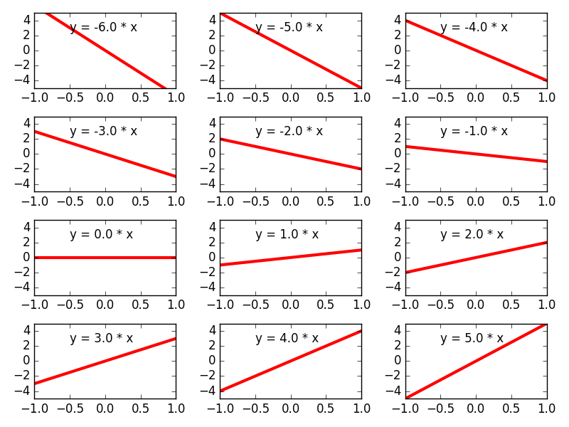
Figure 1. Different values of the parameter w result in different linear equations. The set of all these linear equations is what constitutes the linear model M.
M is a set of all possible models. Choosing a value for w generates a candidate model M(w): y = wx. The regression algorithms that we can write in TensorFlow will iteratively converge to better and better values for the model’s parameter w. An optimal parameter, let’s call it w* (pronounced w star), is the best-fit equation M(w*): y = w*x.
In the most general sense, a regression algorithm tries to design a function, let’s call it f, that maps an input to an output. The function’s domain is a real-valued vector ℝd and its range is the set of real numbers ℝ. The input of the function could be continuous or discrete. However, the output must be continuous, as demonstrated by figure 2.

Figure 2. A regression algorithm is meant to produce continuous output. The input is allowed to be discrete or continuous. This distinction is important because discrete-valued outputs are handled better by classification, which is discussed in the next chapter.
BY THE WAY Regression predicts continuous outputs, but sometimes that’s overkill. Sometimes we just want to predict a discrete output, such as 0 or 1, but nothing in-between. Classification is a technique better suited for such tasks.
We would like to discover a function f that agrees well with the given data points, which are essentially input/output pairs. Unfortunately, the number of possible functions is infinite, so we’ll have no luck trying them out one-by-one. Having too many options available to choose from is usually a bad idea. It behooves us to tighten the scope of all the functions we want to deal with. For example, if we look at only straight lines to fit a set of data points, then the search becomes much easier.
EXERCISE 1 How many possible functions exist that map 10 integers to 10 integers? For example, let f(x) be a function that can take numbers 0 through 9 and produce numbers 0 through 9. One example is the identity function that mimics its input, for example, f(0) = 0, f(1) = 1, and so on. How many other functions exist?
ANSWER 10^10 = 10,000,000,000
How do you know the regression algorithm is working?
Let’s say we’re trying to sell a housing market predictor algorithm to a real estate firm. It predicts housing prices given certain properties, such as number of bedrooms and lot-size. Real estate companies can easily make millions with such information, but they need some proof that it actually works before buying the algorithm from you.
To measure the success of the learning algorithm, you’ll need to understand two important concepts: variance and bias.
- Variance is how sensitive a prediction is to what training set was used. Ideally, how we choose the training set shouldn’t matter – meaning a lower variance is desired.
- Bias is the strength of assumptions made about the training dataset. Making too many assumptions might make it hard to generalize, so we prefer low bias as well.
If a model is too flexible, it may accidentally memorize the training data instead of resolving useful patterns. You can imagine a curvy function passing through every point of a dataset, appearing to produce no error. If that happens, we say the learning algorithm overfits the data. In this case, the best-fit curve will agree with the training data well; however, it may perform abysmally when evaluated on the testing data (see figure 3).
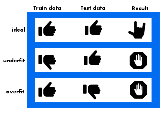
Figure 3. Ideally, the best fit curve fits well on both the training data as well as the test data. However, if we witness it fitting the test data much better than the training data, there’s a chance that our model is underfitting. Lastly, if it performs poorly on the test data but well on the training data, then we know the model is overfitting.
On the other hand, a not-so-flexible model may generalize better to unseen testing data, but would score relatively low in the training data. That situation is called underfitting. A too flexible model has high variance and low bias, whereas a too strict model has low variance and high bias. Ideally we would like a model with both low variance error and low bias error. That way, it both generalizes to unseen data and captures the regularities of the data. See figure 4 for examples.
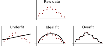
Figure 4. Examples of under-fitting and over-fitting the data.
Concretely, the variance of a model is a measure of how badly the responses fluctuate, and the bias is a measure of how badly the response is offset from the ground-truth. You want your model to achieve both accurate (low bias) as well as reproducible (low variance) results.
EXERCISE 2 Let’s say our model is M(w): y = wx. How many possible functions can you generate if the values of weight parameters w must be integers between 0 and 9 (inclusive)?
ANSWER Only 10. Namely, {y=0, y=x, y=2x, …, y=9x}.
To measure success in machine learning, we partition the dataset into two groups: a training dataset, and a testing dataset. The model is learned using the training dataset, and performance is evaluated on the testing dataset. Out of the many possible weight parameters we can generate, the goal is to find one that best fits the data. The way we measure “best fit” is by defining a cost function.
Linear Regression
Let’s start by creating fake data to leap into the heart of linear regression. Create a Python source file called regression.py and follow along with listing 1 to initialize data. The code will produce an output similar to figure 5.
Listing 1 Visualizing raw input
import numpy as np  //#A
import matplotlib.pyplot as plt  //#B

x_train = np.linspace(-1, 1, 101)  //#C
y_train = 2 * x_train + np.random.randn(*x_train.shape) * 0.33  //#D

plt.scatter(x_train, y_train)  //#E
plt.show()  //#E
#A Import NumPy to help generate initial raw data
#B Use matplotlib to visualize the data
#C The input values are 101 evenly spaced numbers between -1 and 1
#D The output values are proportional to the input but with added noise
#E Use matplotlib’s function to generate a scatter plot of the data
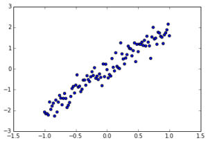
Figure 5. Scatter plot of y = x + noise.
Now that you have some data points available, you can try fitting a line. At the very least, you need to provide TensorFlow with a score for each candidate parameter it tries. This score assignment is commonly called a cost function. The higher the cost, the worse the model parameter will be. For example, if the best fit line is y = 2x, a parameter choice of 2.01 should have low cost, but the choice of -1 should have higher cost.
After we define the situation as a cost minimization problem, as denoted in figure 6, TensorFlow takes care of the inner workings and tries to update the parameters in an efficient way to eventually reach the best possible value. Each step of updating the parameters is called an epoch.
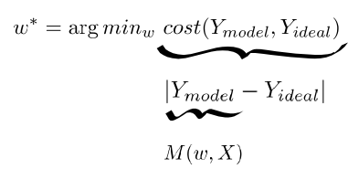
Figure 6. Whichever parameter w minimizes, the cost is optimal. Cost is defined as the norm of the error between the ideal value with the model response. And lastly, the response value is calculated from the function in the model set.
In this example, the way we define cost is by the sum of errors. The error in predicting x is often calculated by the squared difference between the actual value f(x) and the predicted value M(w, x). Therefore, cost is the sum of squared differences between the actual and predicted values, as seen by figure 7.
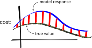
Figure 7. The cost is the norm of the point-wise difference between the model response and the true value.
Let’s update our previous code to look like listing 2. This code defines the cost function, and asks TensorFlow to run an optimizer to find the optimal solution for the model parameters.
Listing 2 Solving linear regression
import tensorflow as tf  //#A
import numpy as np  //#A
import matplotlib.pyplot as plt   //#A

learning_rate = 0.01  //#B
training_epochs = 100  //#B

x_train = np.linspace(-1, 1, 101)  //#C
y_train = 2 * x_train + np.random.randn(*x_train.shape) * 0.33  //#C

X = tf.placeholder("float")  //#D
Y = tf.placeholder("float")  //#D

def model(X, w):  //#E
    return tf.multiply(X, w)

w = tf.Variable(0.0, name="weights")  //#F

y_model = model(X, w)  //#G
cost = tf.square(Y-y_model)  //#G

train_op = tf.train.GradientDescentOptimizer(learning_rate).minimize(cost)  //#H

sess = tf.Session()  //#I
init = tf.global_variables_initializer()  //#I
sess.run(init)  //#I

for epoch in range(training_epochs):  //#J
   for (x, y) in zip(x_train, y_train):  //#K
      sess.run(train_op, feed_dict={X: x, Y: y})  //#L

w_val = sess.run(w)  //#M

sess.close() //#N
plt.scatter(x_train, y_train)  //#O
y_learned = x_train*w_val  //#P
plt.plot(x_train, y_learned, 'r')  //#P
plt.show()  //#P
#A Import TensorFlow for the learning algorithm. We’ll need NumPy to set up the initial data. And we’ll use matplotlib to visualize our data.
#B Define some constants used by the learning algorithm. There are called hyper-parameters.
#C Set up fake data that we will use to find a best fit line
#D Set up the input and output nodes as placeholders since the value will be injected by x_train and y_train.
#E Define the model as y = w*x
#F Set up the weights variable
#G Define the cost function
#H Define the operation that will be called on each iteration of the learning algorithm
#I Set up a session and initialize all variables
#J Loop through the dataset multiple times
#K Loop through each item in the dataset
#L Update the model parameter(s) to try to minimize the cost function
#M Obtain the final parameter value
#N Close the session
#O Plot the original data
#P Plot the best fit line
Congratulations, you’ve just solved linear regression using TensorFlow! Conveniently, the rest of the topics in regression are just minor modifications of Listing 2. The entire pipeline involves updating model parameters using TensorFlow as summarized in figure 8.
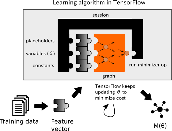
Figure 8. The learning algorithm updates the model’s parameters to minimize the given cost function.
Thanks for reading this crash course in linear regression. To learn more, check out the free first chapter of Machine Learning with TensorFlow and see this Slideshare presentation. You can save 37% with code fccshukla.
About the Author
 Nishant Shukla is a computer vision researcher at UCLA, focusing on machine learning techniques with robotics. He has been a developer for Microsoft, Facebook, and Foursquare, and a machine learning engineer for SpaceX, as well as the author of the Haskell Data Analysis Cookbook.
Don’t forget to save 37% on the book, Machine Learning with TensorFlow with code fccshukla.
