Image Classification, Section 2
Validation Sets for Hyperparameter Tuning
The k-nearest neighbor classifier requires a setting for k. But what number works best? Additionally, we saw that there are many different distance functions we could have used: L1 norm, L2 norm, there are many other choices we didn’t even consider (e.g., dot products). These choices are called hyperparameters and they come up very often in the design of many Machine Learning algorithms that learn from data. It’s often not obvious what values/settings one should choose.
You might be tempted to suggest that we should try out many different values and see what works best. That is a fine idea and that’s indeed what we will do, but this must be done very carefully. In particular, we cannot use the test set for the purpose of tweaking hyperparameters. Whenever you’re designing Machine Learning algorithms, you should think of the test set as a very precious resource that should ideally never be touched until one time at the very end. Otherwise, the very real danger is that you may tune your hyperparameters to work well on the test set, but if you were to deploy your model you could see a significantly reduced performance. In practice, we would say that you overfit to the test set. Another way of looking at it is that if you tune your hyperparameters on the test set, you are effectively using the test set as the training set, and therefore the performance you achieve on it will be too optimistic with respect to what you might actually observe when you deploy your model. But if you only use the test set once at end, it remains a good proxy for measuring the generalization of your classifier (we will see much more discussion surrounding generalization later in the class).
Evaluate on the test set only a single time, at the very end.
Luckily, there is a correct way of tuning the hyperparameters and it does not touch the test set at all. The idea is to split our training set in two: a slightly smaller training set, and what we call a validation set. Using CIFAR-10 as an example, we could, for example, use 49,000 of the training images for training, and leave 1,000 aside for validation. This validation set is essentially used as a fake test set to tune the hyper-parameters.
Here is what this might look like in the case of CIFAR-10:
# assume we have Xtr_rows, Ytr, Xte_rows, Yte as before
# recall Xtr_rows is 50,000 x 3072 matrix
Xval_rows = Xtr_rows[:1000, :] # take first 1000 for validation
Yval = Ytr[:1000]
Xtr_rows = Xtr_rows[1000:, :] # keep last 49,000 for train
Ytr = Ytr[1000:]

# find hyperparameters that work best on the validation set
validation_accuracies = []
for k in [1, 3, 5, 10, 20, 50, 100]:

  # use a particular value of k and evaluation on validation data
  nn = NearestNeighbor()
  nn.train(Xtr_rows, Ytr)
  # here we assume a modified NearestNeighbor class that can take a k as input
  Yval_predict = nn.predict(Xval_rows, k = k)
  acc = np.mean(Yval_predict == Yval)
  print 'accuracy: %f' % (acc,)

  # keep track of what works on the validation set
  validation_accuracies.append((k, acc))
By the end of this procedure, we could plot a graph that shows which values of k work best. We would then stick with this value and evaluate once on the actual test set.
Split your training set into training set and a validation set. Use validation set to tune all hyperparameters. At the end run a single time on the test set and report performance.
Cross-validation. In cases where the size of your training data (and therefore also the validation data) might be small, people sometimes use a more sophisticated technique for hyperparameter tuning called cross-validation. Working with our previous example, the idea is that instead of arbitrarily picking the first 1000 datapoints to be the validation set and rest training set, you can get a better and less noisy estimate of how well a certain value of k works by iterating over different validation sets and averaging the performance across these. For example, in 5-fold cross-validation, we would split the training data into five equal folds, use four of them for training, and one for validation. We would then iterate over which fold is the validation fold, evaluate the performance, and finally average the performance across the different folds.
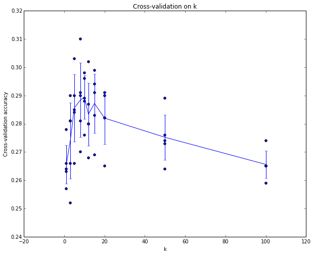
Example of a 5-fold cross-validation run for the parameter k. For each value of k we train on 4 folds and evaluate on the 5th. Hence, for each k we receive five accuracies on the validation fold (accuracy is the y-axis, each result is a point). The trend line is drawn through the average of the results for each k and the error bars indicate the standard deviation. Note that in this particular case, the cross-validation suggests that a value of about k = 7 works best on this particular dataset (corresponding to the peak in the plot). If we used more than five folds, we might expect to see a smoother (i.e., less noisy) curve.
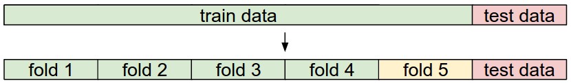
Common data splits. A training and test set is given. The training set is split into folds (for example 5 folds here). The folds 1-4 become the training set. One fold (e.g., fold 5 here in yellow) is denoted as the Validation fold and is used to tune the hyperparameters. Cross-validation goes a step further and iterates over the choice of which fold is the validation fold, separately from 1-5. This would be referred to as 5-fold cross-validation. In the very end once the model is trained and all the best hyperparameters were determined, the model is evaluated a single time on the test data (red).
Pros and Cons of Nearest Neighbor Classifier
It is worth considering some advantages and drawbacks of the Nearest Neighbor classifier. Clearly, one advantage is that it is very simple to implement and understand. Additionally, the classifier takes no time to train, since all that is required is to store and possibly index the training data. However, we pay that computational cost at test time, since classifying a test example requires a comparison to every single training example. This is backwards, since in practice we often care about the test time efficiency much more than the efficiency at training time. In fact, the deep neural networks we will develop later in this class shift this tradeoff to the other extreme: They are very expensive to train, but once the training is finished it is very cheap to classify a new test example. This mode of operation is much more desirable in practice.
As an aside, the computational complexity of the Nearest Neighbor classifier is an active area of research, and several Approximate Nearest Neighbor (ANN) algorithms and libraries exist that can accelerate the nearest neighbor lookup in a dataset (e.g., FLANN). These algorithms allow one to trade off the correctness of the nearest neighbor retrieval with its space/time complexity during retrieval, and usually rely on a pre-processing/indexing stage that involves building a kdtree, or running the k-means algorithm.
The Nearest Neighbor Classifier may sometimes be a good choice in some settings (especially if the data is low-dimensional), but it is rarely appropriate for use in practical image classification settings. One problem is that images are high-dimensional objects (i.e., they often contain many pixels), and distances over high-dimensional spaces can be very counter-intuitive. The image below illustrates the point that the pixel-based L2 similarities we developed above are very different from perceptual similarities:
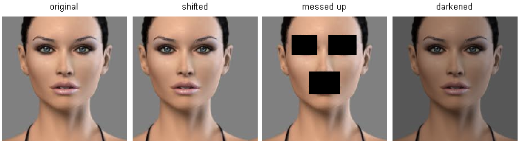
Pixel-based distances on high-dimensional data (and images especially) can be very unintuitive. An original image (left) and three other images next to it that are all equally far away from it based on L2 pixel distance. Clearly, the pixel-wise distance does not correspond at all to perceptual or semantic similarity.
CIFAR-10 images embedded in two dimensions with t-SNE. Images that are nearby on this image are considered to be close based on the L2 pixel distance. Notice the strong effect of background rather than semantic class differences. Click the image for a bigger version of this visualization.
In particular, note that images that are nearby each other are much more a function of the general color distribution of the images, or the type of background rather than their semantic identity. For example, a dog can be seen very near a frog since both happen to be on white background. Ideally we would like images of all of the 10 classes to form their own clusters, so that images of the same class are nearby to each other regardless of irrelevant characteristics and variations (such as the background). However, to get this property we will have to go beyond raw pixels.
In Summary
- We introduced the problem of Image Classification, in which we are given a set of images that are all labeled with a single category. We are then asked to predict these categories for a novel set of test images and measure the accuracy of the predictions.
- We introduced a simple classifier called the Nearest Neighbor classifier. We saw that there are multiple hyper-parameters (such as value of k, or the type of distance used to compare examples) that are associated with this classifier and that there was no obvious way of choosing them.
- We saw that the correct way to set these hyperparameters is to split your training data into two: a training set and a fake test set, which we call validation set. We try different hyperparameter values and keep the values that lead to the best performance on the validation set.
- If the lack of training data is a concern, we discussed a procedure called cross-validation, which can help reduce noise in estimating which hyperparameters work best.
- Once the best hyperparameters are found, we fix them and perform a single evaluation on the actual test set.
- We saw that Nearest Neighbor can get us about 40% accuracy on CIFAR-10. It is simple to implement but requires us to store the entire training set and it is expensive to evaluate on a test image.
- Finally, we saw that the use of L1 or L2 distances on raw pixel values is not adequate since the distances correlate more strongly with backgrounds and color distributions of images than with their semantic content.
In the next segments, we will embark on addressing these challenges and eventually arrive at solutions that give 90% accuracies, allow us to completely discard the training set once learning is complete, and they will allow us to evaluate a test image in less than a millisecond.
Summary: Applying kNN in practice
If you wish to apply kNN in practice (hopefully not on images, or perhaps as only a baseline) proceed as follows:
- Preprocess your data: Normalize the features in your data (e.g., one pixel in images) to have zero mean and unit variance. We will cover this in more detail in later sections, and chose not to cover data normalization in this section because pixels in images are usually homogeneous and do not exhibit widely different distributions, alleviating the need for data normalization.
- If your data is very high-dimensional, consider using a dimensionality reduction technique such as PCA (wiki ref, CS229ref, blog ref) or even Random Projections.
- Split your training data randomly into train/val splits. As a rule of thumb, between 70-90% of your data usually goes to the train split. This setting depends on how many hyperparameters you have and how much of an influence you expect them to have. If there are many hyperparameters to estimate, you should err on the side of having larger validation set to estimate them effectively. If you are concerned about the size of your validation data, it is best to split the training data into folds and perform cross-validation. If you can afford the computational budget it is always safer to go with cross-validation (the more folds the better, but more expensive).
- Train and evaluate the kNN classifier on the validation data (for all folds, if doing cross-validation) for many choices of k (e.g., the more the better) and across different distance types (L1 and L2 are good candidates)
- If your kNN classifier is running too long, consider using an Approximate Nearest Neighbor library (e.g., FLANN) to accelerate the retrieval (at cost of some accuracy).
- Take note of the hyperparameters that gave the best results. There is a question of whether you should use the full training set with the best hyperparameters, since the optimal hyperparameters might change if you were to fold the validation data into your training set (since the size of the data would be larger). In practice it is cleaner to not use the validation data in the final classifier and consider it to be burned on estimating the hyperparameters. Evaluate the best model on the test set. Report the test set accuracy and declare the result to be the performance of the kNN classifier on your data.
