Image Classification, Section 1
We begin by introducing the Image Classification problem, which is the task of assigning an input image one label from a fixed set of categories. This is one of the core problems in Computer Vision that, despite its simplicity, has a large variety of practical applications. Moreover, as we will see later in this series, many other seemingly distinct Computer Vision tasks (such as object detection and segmentation) can be reduced to image classification.
For example, in figure 1, below, an image classification model takes a single image and assigns probabilities to four labels, {cat, dog, hat, mug}. Keep in mind that to a computer, as shown in the figure, an image is represented as one large three-dimensional array of numbers. In this example, the cat image is 248 pixels wide, 400 pixels tall, and has three color channels Red, Green, and Blue (or RGB for short). Therefore, the image consists of 248 x 400 x 3 numbers, or a total of 297,600 numbers. Each number is an integer that ranges from 0 (black) to 255 (white). Our task is to turn this quarter of a million numbers into a single label, such as “cat”.
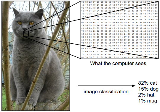
Figure 1. The task in Image Classification is to predict a single label (or a distribution over labels as shown here to indicate our confidence) for a given image. Images are three-dimensional arrays of integers from 0 to 255, of size Width x Height x 3. The 3 represents the three color channels Red, Green, and Blue.
The Challenges
Since this task of recognizing a visual concept (e.g., a cat) is relatively trivial for a human to perform, it is worth considering the challenges involved from the perspective of a Computer Vision algorithm. As we present (an inexhaustive) list of challenges below and in figure 2, keep in mind the raw representation of images as a 3D array of brightness values:
- Viewpoint variation. A single instance of an object can be oriented in many ways with respect to the camera.
- Scale variation. Visual classes often exhibit variation in their size (size in the real world, not only in terms of their extent in the image).
- Deformation. Many objects of interest are not rigid bodies and can be deformed in extreme ways.
- Occlusion. The objects of interest can be occluded. Sometimes only a small portion of an object (as little as few pixels) could be visible.
- Illumination conditions. The effects of illumination are drastic on the pixel level.
- Background clutter. The objects of interest may blendinto their environment, making them hard to identify.
- Intra-class variation. The classes of interest can often be relatively broad, such as chair. There are many different types of these objects, each with their own appearance.
A good image classification model must, therefore, be invariant to the cross product of all these variations, while simultaneously retaining sensitivity to the inter-class variations.
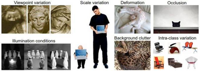
Figure 2.
Taking a Data-driven Approach
How might we go about writing an algorithm that can classify images into distinct categories? Unlike writing an algorithm for, say, sorting a list of numbers, it is not obvious how one might write an algorithm for identifying cats in images. Therefore, instead of trying to specify what every one of the categories of interest look like directly in code, the approach that we will take is not unlike one you would take with a child: we’re going to provide the computer with many examples of each class and then develop learning algorithms that look at these examples and learn about the visual appearance of each class. This approach is referred to as a data-driven approach, since it relies on first accumulating a training dataset of labeled images. Figure 3 shows an example of what such a dataset might look like.
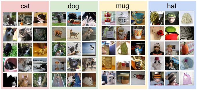
Figure 3. An example training set for four visual categories. In practice we may have thousands of categories and hundreds of thousands of images for each category.
The Image Classification Pipeline
We’ve seen that the task in Image Classification is to take an array of pixels that represents a single image and assign a label to it. Our complete pipeline can be formalized as follows:
- Input: Our input consists of a set of N images, each labeled with one of K different classes. We refer to this data as the training set.
- Learning: Our task is to use the training set to learn what every one of the classes looks like. We refer to this step as training a classifier, or learning a model.
- Evaluation: In the end, we evaluate the quality of the classifier by asking it to predict labels for a new set of images that it has never seen before. We will then compare the true labels of these images to the ones predicted by the classifier. Intuitively, we’re hoping that a lot of the predictions match up with the true answers (which we call the ground truth).
Nearest Neighbor Classifier
As our first approach, we will develop what we call a Nearest Neighbor Classifier. This classifier has nothing to do with Convolutional Neural Networks and it is very rarely used in practice, but it will allow us to get an idea about the basic approach to an image classification problem.
Example Image Classification Dataset: CIFAR-10
One popular toy image classification dataset is the CIFAR-10 dataset. This dataset consists of 60,000 tiny images that are 32 pixels high and wide. Each image is labeled with one of ten classes (for example “airplane, automobile, bird, etc.”). These 60,000 images are partitioned into a training set of 50,000 images and a test set of 10,000 images. In figure 4, below, you can see ten random example images from each one of the 10 classes.
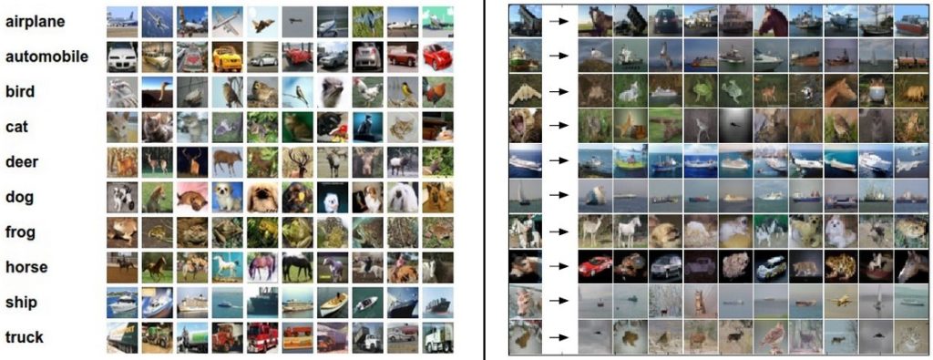
Figure 4. Left: Example images from the CIFAR-10 dataset. Right: first column shows a few test images and next to each we show the top 10 nearest neighbors in the training set according to pixel-wise difference.
Suppose now that we are given the CIFAR-10 training set of 50,000 images (5,000 images for every one of the labels), and we wish to label the remaining 10,000. The nearest neighbor classifier will take a test image, compare it to every single one of the training images, and predict the label of the closest training image. In figure 4, on the right you can see an example result of such a procedure for ten example test images. Notice that in only about three out of ten examples an image of the same class is retrieved, while in the other seven examples this is not the case. For example, in the 8th row the nearest training image to the horse head is a red car, presumably due to the strong black background. As a result, this image of a horse would in this case be mislabeled as a car.
You may have noticed that we left unspecified the details of exactly how we compare two images, which in this case are just two blocks of 32 x 32 x 3. One of the simplest possibilities is to compare the images pixel by pixel and add up all the differences. In other words, given two images and representing them as vectors I1,I2I1,I2 , a reasonable choice for comparing them might be the L1 distance:
d1(I1,I2)=∑p|Ip1−Ip2|d1(I1,I2)=∑p|I1p−I2p|
where the sum is taken over all pixels. Figure 5 shows the procedure visualized.
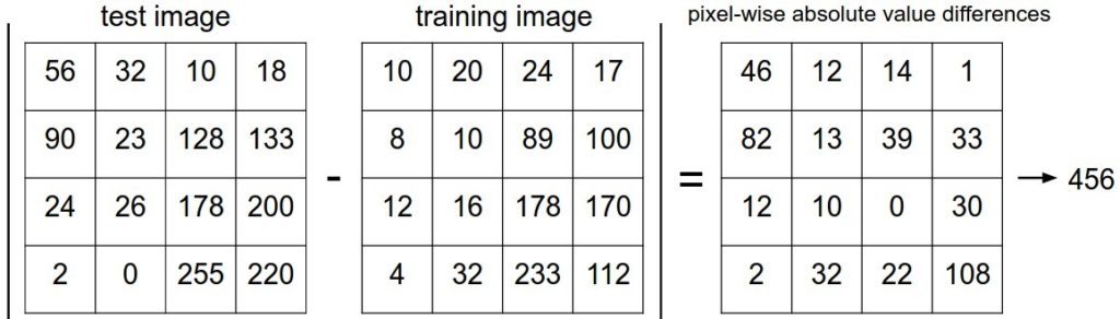
Figure 5. An example of using pixel-wise differences to compare two images with L1 distance (for one color channel in this example). Two images are subtracted elementwise and then all differences are added up to a single number. If two images are identical the result will be zero. But if the images are very different the result will be large.
Let’s also look at how we might implement the classifier in code. First, let’s load the CIFAR-10 data into memory as four arrays: the training data/labels and the test data/labels. In the code below, Xtr (of size 50,000 x 32 x 32 x 3) holds all the images in the training set, and a corresponding 1-dimensional array Ytr (of length 50,000) holds the training labels (from 0 to 9):
Xtr, Ytr, Xte, Yte = load_CIFAR10('data/cifar10/') # a magic function we provide
# flatten out all images to be one-dimensional
Xtr_rows = Xtr.reshape(Xtr.shape[0], 32 * 32 * 3) # Xtr_rows becomes 50000 x 3072
Xte_rows = Xte.reshape(Xte.shape[0], 32 * 32 * 3) # Xte_rows becomes 10000 x 3072
Now that we have all images stretched out as rows, here is how we could train and evaluate a classifier:
nn = NearestNeighbor() # create a Nearest Neighbor classifier class
nn.train(Xtr_rows, Ytr) # train the classifier on the training images and labels
Yte_predict = nn.predict(Xte_rows) # predict labels on the test images
# and now print the classification accuracy, which is the average number
# of examples that are correctly predicted (i.e. label matches)
print 'accuracy: %f' % ( np.mean(Yte_predict == Yte) )
Notice that as an evaluation criterion, it is common to use the accuracy, which measures the fraction of predictions that were correct. Notice that all classifiers we will build satisfy this one common API: they have a train(X,Y) function that takes the data and the labels to learn from. Internally, the class should build some kind of model of the labels and how they can be predicted from the data. And then there is a predict(X) function, which takes new data and predicts the labels. Of course, we’ve left out the meat of things: the actual classifier itself. Here is an implementation of a simple Nearest Neighbor classifier with the L1 distance that satisfies this template:
import numpy as np
class NearestNeighbor(object):

def __init__(self):

pass

def train(self, X, y):
""" X is N x D where each row is an example. Y is 1-dimension of size N """

# the nearest neighbor classifier simply remembers all the training data
self.Xtr = X
self.ytr = y

def predict(self, X):

""" X is N x D where each row is an example we wish to predict label for """
num_test = X.shape[0]

# lets make sure that the output type matches the input type
Ypred = np.zeros(num_test, dtype = self.ytr.dtype)

# loop over all test rows
for i in xrange(num_test):

# find the nearest training image to the i'th test image
# using the L1 distance (sum of absolute value differences)
distances = np.sum(np.abs(self.Xtr - X[i,:]), axis = 1)
min_index = np.argmin(distances) # get the index with smallest distance
Ypred[i] = self.ytr[min_index] # predict the label of the nearest example

return Ypred
If you ran this code, you would see that this classifier only achieves 38.6% on CIFAR-10. That’s more impressive than guessing at random (which would give 10% accuracy since there are ten classes), but nowhere near human performance (which is estimated at about 94%) or near state-of-the-art Convolutional Neural Networks that achieve about 95%, matching human accuracy (see the leaderboard of a recent Kaggle competition on CIFAR-10).
The Choice of Distance
There are many other ways of computing distances between vectors. Another common choice could be to instead use the L2 distance, which has the geometric interpretation of computing the euclidean distance between two vectors. The distance takes the form:
d2(I1,I2)=∑p(Ip1−Ip2)2−−−−−−−−−−−√d2(I1,I2)=∑p(I1p−I2p)2
In other words, we would be computing the pixel-wise difference as before, but this time we square all of them, add them up, and finally take the square root. In numpy, using the code from above, we would need to only replace a single line of code. The line that computes the distances:
distances = np.sqrt(np.sum(np.square(self.Xtr – X[i,:]), axis = 1))
Note that I included the np.sqrt call above, but in a practical nearest neighbor application we could leave out the square root operation because square root is a monotonic function. That is, it scales the absolute sizes of the distances but it preserves the ordering, so the nearest neighbors with or without it are identical. If you ran the Nearest Neighbor classifier on CIFAR-10 with this distance, you would obtain 35.4% accuracy (slightly lower than our L1 distance result).
L1 vs. L2. It is interesting to consider differences between the two metrics. In particular, the L2 distance is much more unforgiving than the L1 distance when it comes to differences between two vectors. That is, the L2 distance prefers many medium disagreements to one big one. L1 and L2 distances (or equivalently the L1/L2 norms of the differences between a pair of images) are the most commonly used special cases of a p-norm.
k – Nearest Neighbor Classifier
You may have noticed that it is strange to only use the label of the nearest image when we wish to make a prediction. Indeed, it is almost always the case that one can do better by using what’s called a k-Nearest Neighbor Classifier. The idea is very simple: instead of finding the single closest image in the training set, we will find the top k closest images, and have them vote on the label of the test image. In particular, when k = 1, we recover the Nearest Neighbor classifier. Intuitively, higher values of k have a smoothing effect that makes the classifier more resistant to outliers (figure 6).
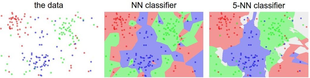
Figure 6. An example of the difference between Nearest Neighbor and a 5-Nearest Neighbor classifier, using 2-dimensional points and 3 classes (red, blue, green). The colored regions show the decision boundaries induced by the classifier with an L2 distance. The white regions show points that are ambiguously classified (i.e., class votes are tied for at least two classes). Notice that in the case of a NN classifier, outlier datapoints (e.g., green point in the middle of a cloud of blue points) create small islands of likely incorrect predictions, while the 5-NN classifier smooths over these irregularities, likely leading to better generalization on the test data (not shown). Also note that the gray regions in the 5-NN image are caused by ties in the votes among the nearest neighbors (e.g., two neighbors are red, next two neighbors are blue, last neighbor is green).
In practice, you will almost always want to use k-Nearest Neighbor. But what value of k should you use? We turn to this problem next.
